Abstract
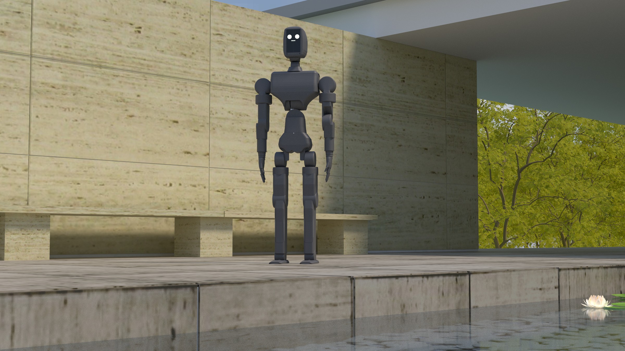
A renderer turns a scene into an image. A differentiable renderer also says how the image would change if the scene did. With path replay, that answer is correct only if the backward pass regenerates the paths the forward pass drew. We describe irys, an open-source spectral path tracer in Rust for the scenes we design (instanced CAD meshes, spectral metals, robots in rooms), whose replay reproduces the forward pass bit for bit.
Its differentiable core is path replay backpropagation on a GPU wavefront. We write each material once as a graph in the tang tensor compiler, and tang lowers it both to GPU kernels and to an f64 CPU reference. An integer random-number generator, fixed-order reductions and a ray-only BVH walk make the replay exact on all 65 536 lanes, and two runs give identical gradients. GPU f32 gradients agree with the f64 reference to . irys also computes pose gradients through instanced CAD meshes (primary edges, an interior term with attached frames, and secondary edges that move shadows and reflections) and a per-vertex image gradient that the vcad BRep kernel pulls back to the dimensions of a part.
We check the GPU’s f32 gradients against the f64 tier, the edge terms against central differences with common random numbers, and the shadows a moving part casts against the same differences with and without the secondary term. Pulled back through vcad’s BRep kernel, irys’s gradient with respect to a part’s dimension agrees with an end-to-end render finite difference to 0.4%. irys also differentiates a diffuse surface’s spectral albedo and each Gaussian splat’s colour and opacity, under the sky, a sun and area emitters, and the GPU tier runs on Vulkan as well as Metal. The remaining limits are that replay is bit-exact per device and driver, pose parameters are rigid, and the secondary-edge term runs on the CPU only. Three checks fall short, and we report them: edge sampling is 5.8% high on one pose parameter of a box, the secondary term passes its check at 64 seeds but not at 256, and the end-to-end CAD finite difference agrees to its step dependence but not to the pullback’s standard error. A companion paper covers inverse problems built on irys, starting with editable CAD from photographs.
1 Introduction
Users judge a renderer first by its images. They judge a differentiable renderer also by its gradients, which say how each pixel would change if a material, a pose or a dimension changed. Those gradients feed optimisers, so an error in them does not show as a wrong pixel. It shows as an optimiser that fails to converge, and the user cannot tell whether the estimator is biased, the device rounded differently, or the samples were noisy.
Path replay backpropagation 1 made physically based differentiable rendering practical by replacing the stored path tape with a second, replayed pass. That only works if the replay regenerates exactly the paths the forward pass drew; otherwise the gradient belongs to a different estimator from the one rendered. Dr.Jit 2 meets this contract by replaying with the same seeded generator, and accumulates parameter gradients with atomic adds whose order can vary between runs. We wanted a GPU tier and an f64 CPU reference that run the same material source and agree to rounding, with each tier bit-identical across runs. A gradient test with fixed random numbers then points at the estimator, not at the replay.
This paper describes irys, the renderer behind vcad and our robotics tools, and how it keeps that contract. Its contributions are:
- One BSDF source, two lowerings, two tiers. Materials are tang tensor graphs. tang lowers each one to an evaluation program and an adjoint program, emitting WGSL kernels for the GPU and running the same graph in its f64 interpreter for the CPU reference. The path logic (ray generation, traversal, bounce, accumulation) is hand-written (Section 3).
- PRB on a deterministic wavefront with hero wavelengths and NEE. The estimator is path replay backpropagation 1 with next-event estimation, as in Mitsuba 3; what we add is a wavefront whose replay and gradient are bit-identical across runs, with no float atomics, with four wavelengths per path and the light-sampled lanes folded into the same graph batch (Section 4).
- Bit-exact replay by construction. The replay is exact because the integer RNG is exact on both tiers, reductions run in a fixed order with no float atomics, and the BVH walk depends only on the ray (Section 5).
- Pose gradients through instanced CAD meshes. irys samples primary edges with crease ownership and visibility-aware importance, differentiates the interior term by forward-mode duals with attached frames, and samples secondary edges for moving shadows and reflections (Section 6).
- Validation at every layer. We check gradients against central differences with common random numbers, and the GPU against the CPU’s f64, on boxes, on a shaded robot arm read from its CAD source, and on the shadows it casts (Section 7).
- Gradients for CAD parameters. irys computes a per-vertex image gradient that the vcad BRep kernel pulls back to the dimensions of the part. vcad’s paper 3 shares it as a benchmark (Section 7.5).
1.1 Scope and limits
- Determinism is per device and driver. The GPU tier runs in f32, so its results agree with the f64 reference to rounding, not bitwise; it is bit-identical against itself on one device and driver.
- Materials. The differentiable materials are a GGX conductor with a three-band spectral Fresnel, a diffuse surface’s three-band spectral albedo, and each Gaussian splat’s 4 DC colour and base opacity (Section 7.3). irys does not differentiate the environment or a splat’s position or shape. On the GPU a replay records at most 256 splat crossings per path.
- Lights. The emitters are the environment (a sky and a von Mises–Fisher sun lobe) and area emitters, sampled with next-event estimation and multiple importance sampling on both tiers.
- Pose parameters are rigid. Joint angles and the camera move instances rigidly. Non-rigid shape change enters only through the BRep pullback of Section 7.5.
- No comparison with Mitsuba 3 here. Every check in this paper is internal, against irys’s own f64 tier and central differences. The repository has an earlier comparison with Mitsuba 3 (
bench/mitsuba), measured on different hardware and not repeated in this paper’s run. - Hardware. The GPU tier runs on Metal and on Vulkan. Every number in this paper comes from one run on one machine: an NVIDIA RTX 4090 through Vulkan, with 12 vCPUs of an AMD EPYC 7K62 for the CPU tier (Section 9). We have not measured timings on other GPUs.
2 Background and related work
Differentiable path tracing. Li et al. introduced edge sampling to account for visibility discontinuities in Monte Carlo rendering 5. Radiative backpropagation 6 and path replay backpropagation 1 reduced the memory of the adjoint pass to a constant per path. Zeltner et al. classify estimators for differential transport as attached or detached 7, the vocabulary we use. Dr.Jit provides a tracing compiler for such methods 2, on which Mitsuba 2 and 3 are built 8,9. Path-space differentiable rendering derives the boundary term as an integral over path space 10. Rasterization-based differentiable renderers trade global illumination for speed 11. Other methods handle visibility by reparameterisation 12, warped-area sampling 13 or projective sampling 14. We compared warped estimators for the secondary term and chose edge sampling (Section 6).
Spectral rendering. Hero wavelength sampling 15 traces several wavelengths along one path, the hero choosing directions. We use it unchanged and make each wavelength its own PRB lane.
Compilers for rendering. SLANG.D adds automatic differentiation to a shading language 16 and is the closest analogue to writing BSDFs as tang graphs. Laine et al. argue for splitting a path tracer into wavefront kernels 17, the structure we use.
Differentiable rendering systems. Mitsuba 3 9 implements path replay with next-event estimation and multiple importance sampling, projective sampling and reparameterisation on Dr.Jit, and is the closest system to irys’s differentiable core. irys differs in what it guarantees rather than in the estimator: a replay that is bit-identical to the forward pass by construction, an f64 reference that runs the same material source, spectral transport with hero wavelengths, and visibility terms adapted to CAD tessellations (coplanar slivers, crease ownership, attached frames).
Inverse CAD and measurement from images. Recovering an editable CAD description from observations is usually posed as program synthesis over meshes, point clouds or drawings 18–20, and close-range photogrammetry measures manufactured parts by triangulating targets and features 21. For photographs, irys adds what both lack, the gradient of a rendered image with respect to a part’s pose, finish and dimensions. Our companion paper’s BRep kernel 3 differentiates the CAD parameters upstream of the mesh, and Section 7.5 joins it to irys.
3 Materials as compiled graphs
The differentiable material has parameters : GGX roughness with height-correlated Smith masking, and a Schlick Fresnel whose is interpolated between three spectral hats. We write it once as a tang TensorGraph whose inputs are per-lane columns (the cosines at a vertex and the hero wavelength’s hat weights) and whose is broadcast. tang lowers it two ways. The eval program returns and its pdf. The adjoint program is the backward pass of , so the batch sum over lanes is the reduction to . tang emits each program as WGSL, one kernel per materialised comprehension, or as compiled C in f32 and an interpreter in f64 for the CPU. The interpreter matches a hand-written f64 GGX to , and the compiled C matches the interpreter to in the worst relative error.
The path logic is hand-written, in WGSL for the GPU and in Rust for the CPU reference: ray generation, BVH traversal, bounce, the throughput update, the final splat and accumulation, and the device-side loss scoring. tang’s comprehensions are straight-line bodies over fixed shapes, so they cannot express data-dependent path loops or a traversal stack today. Sampling the GGX visible normals is detached, since it needs no derivative under PRB, and the divisor pdf is the sampler’s, which we test against the graph’s pdf to .
4 Path replay on a wavefront
Estimator. For a path with vertices and radiance , BSDF-only PRB accumulates at each vertex, where is the radiance collected before vertex . With next-event estimation and multiple importance sampling the gradient becomes
where is the BSDF-sampled direction, the light-sampled one, the NEE contribution at and the radiance up to and including it. We detach the pdfs in the MIS weights, so the weights are constants under ; this keeps the estimator unbiased because the weights still sum to one for every path. In the wavefront the light-sampled lanes are the second half of one graph batch, so a single adjoint dispatch serves both strategies. A nonlinear loss needs the primal image before the adjoint, so irys scores the loss between the forward and replay passes.
Hero wavelengths. Each path carries four stratified wavelengths, the hero and its rotations by of the visible range 15. Only the hero draws directions. The wavefront’s lanes are (path, wavelength) pairs, four times as many as paths, and each lane is its own PRB path. At equal paths, four wavelengths cut per-pixel variance 7.4× in total and 28.7× in chroma. That costs four times the lanes, so per lane the gain is 1.9× in total and 7.2× in chroma.
Memory. PRB stores nothing per vertex. With four wavelengths a path costs about 71 f64 words at depth 2 and at depth 8 alike. Memory scales with paths, not pixels. irys traces frames larger than one dispatch in chunks, and a 1024² image at 4 spp, 16 777 216 lanes, replays bit-identically in 9 chunks.
5 Determinism
PRB’s replay must redraw the forward pass’s paths. irys makes this hold in four ways.
- Same pipelines. Forward and replay dispatch the same compute pipelines over the same bind groups; they differ only in a uniform that enables the store of .
- An integer RNG on both tiers. SplitMix64 is ported onto pairs of 32-bit words built from 16-bit limbs, so the GPU, which lacks 64-bit integers, produces exactly the CPU’s stream. A uniform keeps the top 24 of 53 bits, so both tiers walk the same paths up to f32 rounding of the geometry.
- No float atomics. The reduction over lanes is tang’s monoid reduction, split 256 ways with one workgroup per parameter and a fixed combining tree. Splat accumulation runs in bounce order, loss scoring uses a fixed stride and tree, chunks are summed in order, and the device prefix sum used by edge sampling has a fixed order.
- A walk that depends only on the ray. BVH traversal uses a fixed-size stack, visits the near child first by slab entry with a deterministic tie-break, and culls by the closest hit so far. The walk, and therefore the floating-point sequence, is a function of the ray alone, not of thread scheduling.
The result is that the replay reproduces the forward radiance bit for bit on all 65 536 lanes at depths 2 and 8, with NEE, and through the two-level instanced scenes and a garden scene of meshes and Gaussian splats; two runs give bitwise-identical loss and . The guarantee holds per device and driver. A different GPU or compiler may round differently, and then agrees with the CPU reference only to f32 precision.
6 Pose gradients through instanced CAD
Scenes. A scene is a two-level BVH: one bottom-level tree per CAD part or group, and a top-level tree over instances, each with an object-to-world transform. irys maps rays into an instance’s space without renormalising them, so hit distances compare across instances. A pose , such as joint angles, is a map from parameters to the transforms of the moving instances. The full robot in this paper has 2.4 million triangles, tessellated by vcad from its CAD source (a text format of parametric solids).
Primary edges. Moving an instance moves the curves across which the radiance arriving at the camera plane jumps: silhouettes, boundaries and creases between faces that are not coplanar. By Reynolds transport, a pixel’s derivative includes
over the projected edges , where is the edge’s outward normal and the normal speed of the material point under 5. We sample edges with density proportional to screen length times an importance (1 for silhouettes, a dihedral weight for creases, a small weight for back-facing edges), trace the two sides pixels apart with common random numbers, and require the inner ray to hit the edge’s own triangle or a coplanar neighbour. CAD tessellations contain many slivers thinner than , and without the coplanar rule the estimator loses most silhouette samples. The face that meets the eye more squarely owns a crease between two front faces, so the estimator counts its jump once. A low-resolution buffer of which instance each pixel sees lets the sampler demote edges it shows hidden, which cut variance 2× at equal samples. Sampling runs on the device, with a fixed-order prefix sum; it took the edge term on the arm from 273 ms to 15.3 ms per iteration. The device sampler is biased low on the full robot by a few percent, so the robot checks below use host samples (Section 8).
Interior term and attached frames. Away from discontinuities the estimator is smooth in at fixed random numbers, and we differentiate it by forward-mode dual numbers through a re-trace of the frame: ray–triangle intersection with the corners as duals, the shading frame, GGX sampling and evaluation, NEE and the MIS weights. The renderer builds a vertex’s tangent frame from its normal with a construction that flips sign when the normal crosses a plane, a discontinuity in at fixed random numbers that no edge term sees. We instead differentiate the estimator whose frame on a moving instance is rigidly attached, . At it is the rendered estimator exactly, and for every it is an equally valid estimator of the same image, so, wherever the integrand is smooth in and differentiation passes under the integral, its derivative is an unbiased estimate of from the paths the forward pass already drew; the edge terms handle the discontinuities where it does not. The duals reproduce the forward pass’s values to .
Secondary edges. When an instance moves, its shadow and its reflection move too. As in Li et al. 5, we sample the edges seen from each path vertex with a hierarchy over edges, here a per-tree edge BVH, under one-sample multiple importance over three densities: geometric, toward the sun’s cone, and toward the mirror lobe. The boundary term includes the velocity of the BSDF-sampled direction, obtained by inverting the sampler at the path’s random numbers and redrawing it in duals. Against the best setting of a warped-area estimator on the same configuration, at about the same cost per estimate, edge sampling had at least 21× lower variance on every parameter.
Camera. The same machinery differentiates a seven-parameter camera (translation, rotation, field of view), with the eye, axes and field of view as duals and every instance’s edges as candidates. This paper reports no check of the camera gradient.
7 Results
Unless stated, we check gradients against central differences (CD) of the same estimator with common random numbers; “frozen” means the random numbers are fixed so the CD is noise-free. Monte Carlo comparisons report a z-score, the difference over its standard error. Timings are release builds on the RTX 4090 machine above. The number in each table is read from data/measured.tsv, whose rows give the source test and commit.
7.1 Correctness of the material gradient
data/measured.tsv.| Check | Configuration | Result |
|---|---|---|
| CPU f64 PRB vs frozen CD | BSDF-only, four θ, 4 λ | – |
| same, NEE + MIS | two instanced boxes | ≤ |
| GPU f32 vs CPU f64, radiance | median / p99 per lane | / |
| GPU f32 vs CPU f64, loss | 32×32×4 | |
| GPU f32 vs CPU f64, δθ | worst parameter | |
| same with NEE | radiance p99 / worst δθ | / |
| Replay vs forward | 64×64×4×4 λ, depth 2 and 8 | all 65 536 bit-identical |
7.2 Variance and throughput
At equal samples per pixel, NEE with MIS lowers per-pixel variance 7.5× against BSDF sampling alone on a scene of two instanced boxes, with image means agreeing within noise. A gradient of the 96×96, 8 spp frame at depth 4 (73 728 paths, four wavelengths each) costs a median of 1.1 ms on the GPU without NEE (1.06–4.67 ms over four runs; the slowest run is the first, which includes pipeline compilation) and 3.88 ms with NEE (2.61–5.51 ms). The forward pass alone takes a median of 0.82 ms, about 89 million paths per second, so the replay and adjoint add 0.27 ms; NEE doubles the batch. The same gradient through the CPU tier’s compiled C costs a median of 555 ms (551–608 ms), measured in a separate test against the GPU gradient with the loss scored on the device, 1.04 ms (median of four runs), so the GPU tier is about 532× faster end to end on this machine. This compares irys with itself; it is not a comparison with another renderer.
7.3 Diffuse albedo, splats and emitters
The same replay differentiates two more kinds of parameter. A Lambertian BSDF is linear in its albedo, so a diffuse vertex adds to band of the albedo’s gradient, with the radiance before the vertex. A splat’s colour is linear too. Its opacity also scales everything behind it, so , where is the path throughput at the segment, the transmittance in front of splat , its colour, the emission composited behind it on the segment and the light beyond the segment. On the GPU the replay writes one record per splat crossed and the host sums the records in a fixed order, so there are still no float atomics. Area emitters with next-event estimation and multiple importance sampling run on both tiers, and their 16 gates pass on Vulkan.
data/measured.tsv.| Parameter | CPU f64 vs CD | GPU f32 vs CPU f64 | Replay lanes identical |
|---|---|---|---|
| diffuse albedo, three bands | all 65 536 | ||
| splat colour and opacity | all 65 536 |
7.4 Pose gradients
On a box against the sky, where the edge term is the whole derivative, edge sampling matches CD on two of its three pose parameters (z = 0.29 and 0.04). On the third it is 5.8% high (z = 3.41), in every run we have made; the test’s gate, four standard errors plus 3% of the reference, passes, but we have not found the cause. The device’s f32 edge term matches the CPU’s f64 to . On the shaded arm over a floor, the edge and interior terms alone miss CD by z = 3.56, −4.71, 3.71. The secondary term, mostly the arm’s shadow on the floor, is 13%, 34% and 23% of the three derivatives. With secondary edges the same check gives z = 0.23, −0.71, 0.39 at 64 seeds; at 256 seeds the check fails, because the secondary estimate is heavy-tailed (Section 8).
7.5 From pixels to CAD parameters
The edge sampler’s velocity is a projection of the material point’s motion, so replacing the pose’s velocity with a unit translation per axis yields for every mesh vertex. vcad’s differentiable seam 3 takes that cotangent on the nodes of a frozen tessellation and returns the derivative with respect to a CAD parameter in one reverse pass. The shared benchmark uses rose’s left shoulder-pitch output plate, a 3 mm rounded plate with a 49 mm bearing bore and twelve bolt holes, with the bore diameter. irys renders vcad’s frozen tessellation unchanged (4 942 nodes, 9 932 triangles). This is the mesh whose connectivity the kernel holds fixed while it differentiates node positions. The render is against the sky at 160×128, under a fixed smooth image loss.
9155391, vcad d10f279, rose 832192f. The pullback’s error is the Monte Carlo standard error over 8 edge-sampling seeds of 100 000 samples. The render FD moves the plan’s nodes along vcad’s FD velocities; it varies by about 0.5% between and mm, so the pullback agrees with it within the FD’s own step dependence, though not within the pullback’s standard error. The same numbers appear in vcad’s paper 3.| Path to dL/dθ | Value | vs pullback |
|---|---|---|
| vcad pullback of irys’s | 40.17 ± 0.0226 | – |
| vcad forward seam, | 40.17 | |
| vcad finite-difference node velocities | 40.17 | |
| End-to-end render FD ( mm) | 40.01 |
A finite difference that rebuilds the part is not a usable reference here. Rebuilding at loses node correspondence for mm and changes topology at mm, where the bore rim’s segment count, chosen from the circle’s size, drops by one; below that the render difference is quadrature noise. The pullback has no step size. It is exact for the frozen mesh, and irys’s sampling error is the only noise in the result.
8 Discussion
Why insist on bit-exact replay. With an exact replay, a gradient that disagrees with its reference is a bug in the estimator, not an artefact of the replay. We could therefore set most gates tight and debug failures by bisection; the box edge test is the exception, with a gate loose enough to pass a 5.8% discrepancy we have not explained. That is how we found the crease-ownership bug in our first edge sampler. It inflated one parameter’s edge term by a factor of five on a shaded arm while the mask-only test passed.
The f64 reference. Running the same tang graph in f64 on the CPU separates three error sources that are otherwise entangled: estimator bias (CPU against frozen CD), device rounding (GPU against CPU), and Monte Carlo noise (live sampler against CD over seeds).
Future work: from photographs to CAD programs. This paper validates gradients; it does not use them to recover anything. Their use is in inverse problems, and the hardest is recovering the model itself. Given a few photographs of a part, the task is to find the editable CAD program, its features and their dimensions. irys’s gradients make the dimensions tractable inside such a search, and a printed tag fixes the camera and the scale. The open problem is topology, meaning which features the part has. We take that up in a companion paper 22, which evaluates the search on held-out parts and reports where it fails. One photograph is often not enough, and a small residual does not mean the features are right.
Remaining gaps. The secondary term runs on the CPU in f64 and costs about a quarter of an iteration; the shaded-arm check passes at 64 seeds but not at 256. Rare large samples dominate its variance, but we have not ruled out a bias. Edge sampling is 5.8% high on one pose parameter of the box, and the device edge sampler is biased low on the full robot by a few percent (from earlier runs; not in data/measured.tsv), both for causes we have not found; the robot checks use host samples. The adjoint’s reduction is not fused. Splat gradients cover colour and opacity only, and the GPU replay sums their records on the host. The look renderer’s hair tests fail on Vulkan; they are not on the differentiable path. Timings are from one GPU only.
9 Reproducibility
irys is open source under Apache-2.0, and its crates are on crates.io. paper/irys/repro/repro.sh clones irys and the rose CAD at pinned commits, runs every gate test and the two robot-arm examples in the release profile, and writes data/measured.tsv; each row names the test or example that measured it. Every measured number in this paper comes from one such run at irys 9155391 on 2026-11-12, on the machine in data/env.tsv; the raw log is data/raw/tests.log. Design facts (the robot’s triangle count, the true and initial poses) come from data/constants.tsv, and a few tolerances and observations quoted in the text come from the irys sources and design log. The same run also executes the robot-arm pose fit, which diverged on this machine; this paper uses none of its numbers.
10 Conclusion
Path replay gives the gradient of the rendered image only if the replay regenerates the forward pass. irys makes the replay exact by construction. An integer random-number generator, fixed-order reductions and a ray-only traversal reproduce the forward pass bit for bit. Materials compile from one graph to a GPU tier and an f64 reference. Pose and shape gradients pass through instanced CAD meshes to the dimensions in the model. We check the material, pose and shape gradients against independent references, and report the three checks that fall short. The companion paper covers what those gradients can recover, starting with editable CAD from photographs. irys is open source.
References
- 1. Vicini, D., Speierer, S. & Jakob, W. Path Replay Backpropagation: Differentiating Light Paths using Constant Memory and Linear Time. ACM Transactions on Graphics 40, (2021).
- 2. Jakob, W., Speierer, S., Roussel, N. & Vicini, D. Dr.Jit: A Just-In-Time Compiler for Differentiable Rendering. ACM Transactions on Graphics 41, (2022).
- 3. Pedersen, C. Exact Gradients Through a BRep Kernel. (2026).
- 4. Kerbl, B., Kopanas, G., Leimkühler, T. & Drettakis, G. 3D Gaussian Splatting for Real-Time Radiance Field Rendering. ACM Transactions on Graphics 42, (2023).
- 5. Li, T.-M., Aittala, M., Durand, F. & Lehtinen, J. Differentiable Monte Carlo Ray Tracing through Edge Sampling. ACM Transactions on Graphics 37, (2018).
- 6. Nimier-David, M., Speierer, S., Ruiz, B. & Jakob, W. Radiative Backpropagation: An Adjoint Method for Lightning-Fast Differentiable Rendering. ACM Transactions on Graphics 39, (2020).
- 7. Zeltner, T., Speierer, S., Georgiev, I. & Jakob, W. Monte Carlo Estimators for Differential Light Transport. ACM Transactions on Graphics 40, (2021).
- 8. Nimier-David, M., Vicini, D., Zeltner, T. & Jakob, W. Mitsuba 2: A Retargetable Forward and Inverse Renderer. ACM Transactions on Graphics 38, (2019).
- 9. Jakob, W. et al. Mitsuba 3 renderer. https://mitsuba-renderer.org/ (2022).
- 10. Zhang, C., Miller, B., Yan, K., Gkioulekas, I. & Zhao, S. Path-Space Differentiable Rendering. ACM Transactions on Graphics 39, (2020).
- 11. Laine, S. et al. Modular Primitives for High-Performance Differentiable Rendering. ACM Transactions on Graphics 39, (2020).
- 12. Loubet, G., Holzschuch, N. & Jakob, W. Reparameterizing Discontinuous Integrands for Differentiable Rendering. ACM Transactions on Graphics 38, (2019).
- 13. Bangaru, S. P., Li, T.-M. & Durand, F. Unbiased Warped-Area Sampling for Differentiable Rendering. ACM Transactions on Graphics 39, (2020).
- 14. Zhang, Z., Roussel, N. & Jakob, W. Projective Sampling for Differentiable Rendering of Geometry. ACM Transactions on Graphics 42, (2023).
- 15. Wilkie, A., Nawaz, S., Droske, M., Weidlich, A. & Hanika, J. Hero Wavelength Spectral Sampling. Computer Graphics Forum (Proc. Eurographics Symposium on Rendering) 33, (2014).
- 16. Bangaru, S. P. et al. SLANG.D: Fast, Modular and Differentiable Shader Programming. ACM Transactions on Graphics 42, (2023).
- 17. Laine, S., Karras, T. & Aila, T. Megakernels Considered Harmful: Wavefront Path Tracing on GPUs. in High-Performance Graphics (2013). doi:10.1145/2492045.2492060.
- 18. Sharma, G., Goyal, R., Liu, D., Kalogerakis, E. & Maji, S. CSGNet: Neural Shape Parser for Constructive Solid Geometry. in IEEE/CVF Conference on Computer Vision and Pattern Recognition (CVPR) 5515–5523 (2018).
- 19. Du, T. et al. InverseCSG: Automatic Conversion of 3D Models to CSG Trees. ACM Transactions on Graphics 37, (2018).
- 20. Ellis, K., Ritchie, D., Solar-Lezama, A. & Tenenbaum, J. B. Learning to Infer Graphics Programs from Hand-Drawn Images. in Advances in Neural Information Processing Systems (NeurIPS) vol. 31 (2018).
- 21. Luhmann, T., Robson, S., Kyle, S. & Boehm, J. Close-Range Photogrammetry and 3D Imaging. (De Gruyter, 2019).
- 22. Pedersen, C. Seeing Is Measuring: Editable CAD programs from photographs. (2026).